Latest News
- Clues beginning to emerge on asymtomatic SARS-CoV-2 infection
- Back in November of 2020, during the first wave of the COVID-19 pandemic, I was teaching an in-person microbiology laboratory. One of my students had just been home to see his parents, and they all c…
- Read more
- Could there maybe be better uses of genetics and probiotics?
- Professor Meng Dong and his laboratory have created a probiotic that can metabolize alcohol quickly and maybe prevent some of the adverse effects of alcohol consumption. The scientists cloned a highl…
- Read more
- ChatGPT is not the end of essays in education
- The takeover of AI is upon us! AI can now take all our jobs, is the click-bait premise you hear from the news. While I cannot predict the future, I am dubious that AI will play such a dubious role in…
- Read more
- Fighting infections with infections
- Multi-drug-resistant bacterial infections are becoming more of an issue, with 1.2 million people dying of previously treatable bacterial infections. Scientists are frantically searching for new metho…
- Read more
- A tale of two colleges
- COVID-19 at the University of Wisconsin this fall has been pretty much a non-issue. While we are wearing masks, full in-person teaching is happening on campus. Bars, restaurants, and all other busine…
- Read more
Chapter 30 - Microbial Methods
30 - 1 Culturing Bacteria
To study microorganisms and their metabolism, it is almost always desirable to bring them into the laboratory and grow them under controlled conditions. This is largely because it is necessary to have pure cultures (that is growth of only one unique type of microorganism) to be confident about assigning a characteristic or behavior to that single species. Therefore, it is necessary to create conditions where an individual microbe can grow free from other living organisms. How do scientists create suitable nutrient conditions so that microorganisms will grow? Then, once you get a group of microbes growing from a certain environment, how do you separate them from one another and create pure cultures? These are the classic methods of microbiology that were developed in the 19th century by the early microbiologists. In this section we will examine these techniques and talk about a few practical aspects of making media and isolating microbes.
Making media and sterilization
We described different types of media and some of their formulations in Chapter 5 on Bacterial Nutrition. These formulations provide all the necessary nutrients that the appropriate microorganism needs to multiply. We also talked about the critical aspect of medium sterilization in Chapter 5. It is critical to remove all other life forms from a prepared medium before inoculation with the microbe to be studied if one wants to obtain interpretable results.
While it may seem at first to be a daunting task to prepare and sterilize medium, it turns out to be quite easy. In most cases media making involves dissolving the ingredients in water, adjusting the medium to the correct pH and autoclaving. If you can prepare a cake from a box mix, you have all the skills you need to successfully make growth medium. Of course, a deeper understanding about the ingredients in a medium (their nutritional role, their heat stability, which ones will react with one another at high temperature, etc.) is useful, especially in formulating a new medium or trying to troubleshoot the failure of a microbe to grow. The nuances of media-making are beyond the scope of this book, but any good introductory microbiology laboratory course will have this information.
Once a sterile medium is prepared, it is also necessary to keep unwanted microorganisms in the environment from contaminating it during handling. Such methods were developed that prevent microbes from entering a medium and these methods are collectively called aseptic technique. These procedures consist of using various barriers to prevent unwanted microbes from entering medium and making quick transfers of desirable microbes. While keeping microbes out may seem like a job for high tech equipment, it again is quite simple. In most cases flasks and tubes are capped with a cotton or foam plug or covered with a loose fitting cap or even aluminum foil. Plates of solid medium have a lid that covers the agar. For the transfer of microbes, a wire often with a loop at the end is used. Just before transfer the wire is heated to kill any microorganisms present. The loop is cooled for a few seconds and then dipped in a growth of microbes. This is then passed through the medium to be inoculated and after transfer the loop is heated again. As much as possible, the area where work is to be done is kept free of microorganisms using disinfectant and controlled airflow. Figure 30.1 contains a movie that demonstrates the most common procedures used in aseptic technique.
Figure 30.1. Flame sterilization and tube-to-tube transfer. This movie describes the techniques necessary for transferring microbes safely from one medium to another. They are simple techniques, but have to be practiced compulsively to ensure no contamination of the sample or the environment.
Isolating microorganisms
The extraction of a microorganism from its environment and into pure culture would seem a daunting task and it was difficult for many years after people discovered and tried to culture microbes. However, easy techniques were eventually developed that greatly simplified the isolation of pure cultures.
One important development was the formulation of solid medium and the most common solidifying agent used in microbiology is agar. Agar is a polysaccharide extracted from seaweed that has some very useful properties. When suspended in water and heated to 100 °C it melts and forms a slightly viscous solution. Agar remains molten until the temperature drops below 45°C at which point it solidifies, forming a Jello-like material. Once solidified, it will not melt until again heated to 100°C. This allows the cultivation of microorganisms at a wide range of temperatures. In addition, its lower solidification point permits the addition of heat labile compounds to media before its final distribution. By mixing agar with a liquid nutrient medium, a Jello-like material forms that can be poured into tubes or shallow dishes (called Petri plates) to create surfaces for microbes to grow on. If one places a single bacterium of most species on this solid surface, it will stay in one place and be unable to move about. Assuming the medium supports growth the microbe makes a number of identical clones of itself and these pile up on top of one another. After long enough incubation these become visible to the naked eye and form a colony. These colonies are populations of a single type of microorganism and thus achieve the stated goal, a pure culture. The question then becomes, how do you deposit a single bacterium onto the solid surface and the answer is amazingly easy. One simply dips a thin instrument, such as a metal inoculating loop or a sterile stick, into a source of microbes and then rubs it across the agar. The mechanical force of rubbing the loop or stick causes microorganisms to fall off and be deposited on the agar. By streaking in several phases, it is possible to get areas of the agar where individual bacteria have fallen off the loop and resulted in formation of isolated colonies. Now it is always possible that two different cell types happened to land on the same spot, so that the colony you see has a mixture of the progeny of both. So to be confident that you really have a pure isolate, one often restreaks colonies a second time before choosing one colony to work with. Figure 30.2 demonstrates the process of streak plates and media preparation.
Figure 30.2. Streak plates and media making. Streak plates are an easy way of mechanically separating microbes in a growth. To achieve this a sterile loop is rubbed across the surface of an agar plate.
It is also possible to obtain individual colonies by using dilution plating. A culture is repeatedly diluted in an appropriate buffer solution until a low enough concentration of cells is reached. Spreading or pouring a portion of this dilution onto a plate separates the bacteria into individual connected groups with each group of bacteria typically containing just one or hopefully no more than a few cells of a single organism. See below under viable plate counts for more on this.
Anoxic conditions
Either for isolation or for subsequent analysis, it is often important to culture microbes under a gas phase that is different from that of the normal atmosphere. Though this does not refer exclusively to the removal of O2, that is such a common issue in microbiology that we will deal with that first and at greatest depth.
There are two general classes of anaerobes: obligate (or stringent) and aeroltolerant (or nonstringent). The latter can tolerate low levels of O2 for brief periods, but the former cannot. Obviously methods for handling the former group will also work for the less sensitive aerotolerant class. The standard method for handling obligate anaerobes employs an anoxic chamber, which is a flexible plastic box with gloves built into the walls so that samples can be manipulated from the outside. The internal atmosphere is maintained through the use of special gas mixes and always involves 5-10% H2. Except for H2, gasses are scrubbed of trace levels of O2 with a palladium catalyst. Samples are added and removed from the chamber through an airlock, which is a small chamber that separately opens to both the outside and the main chamber. In this way, media, tubes and bottles can be added to the airlock, the O2 removed, and then admitted to the chamber. After manipulation, the sealed bottles and tubes can be removed from the chamber through the airlock. Alternatively, samples can be incubated within the chamber itself.
Aerotolerant organisms can be handled in this way as well, but can often be handled on the bench top but with procedures that minimize the amount of O2 exposure. This might include minimizing the amount of culture surface exposed to the air, blowing inert gases over open vessels or including reducing agents in the media to remove dissolved O2.
Facultative microbes are also examined under anoxic conditions, but here the exposure of the organism to O2 is not critical. Such anaerobic environments can be created through the use of sealable jars that can hold a dozen Petri plates. These can be made anaerobic through the use of commercially available gas generators that produce H2 and CO2 (and remove O2) after water is added. Alternatively jars, bottle or tubes can be made anoxic by repeated vacuum evacuation and flushing with an inert gas. This also allows the introduction of a specific gas environment.
30 - 2 Counting microorganisms
There are many different reasons one might need to known the population of microorganisms in a given sample. For example, determining the rate at which a microbe is killed by UV light requires analysis of the number of viable cells before, and at various times during, UV exposure. In other experiments, it is important to know that you have the right density or growth stage to use, such as required for transforming a plasmid constructed in vitro into an E. coli strain. Assessment of bacterial populations in applied industries is also important. Many food-processing plants measure the level and type of microorganisms present in their food by doing counts on selective medium. Also, sewage treatment plants routinely sample and count the microbes present in their treatment systems to insure the correct type and numbers of bacteria are present. The microbial count can be determined using a wide array of techniques. Note that these assays all require somewhat different information and work over different time frames, as explained below. In this section we summarize some of the more common methods.
Microscopic counts
The most direct method of counting microorganism is by the use of a microscope and a slide with special chambers of known volume. These slides allow the counting of a small number of cells in a small volume and extrapolating the result to determine the population. An example of such a device is shown in Figure 30.3. A culture is placed on the slide marked with precise grids. The number of cells present in each grid is counted and an average determined. Conversion using a formula gives the number of cells per milliliter in the culture. This method is rapid, a result can be known in just a few minutes, and is easy to perform. However without the use of special viability stains, it is impossible to distinguish living cells from dead ones. If this distinction is important, direct microscopic counts are not the solution. Finally, cultures containing less than 1 million cells per ml are actually too dilute for direct counts since there are too few cells in the very small volume that is actually examined under the microscope for an accurate count.
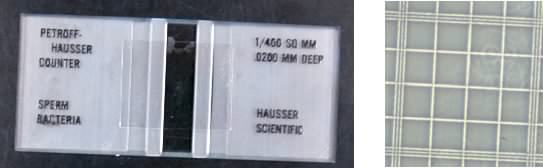
Figure 30.3. A Petroff-Hausser counting chamber. By carefully counting the microbes in each square, it is possible to accurately determine the population of microbes in a sample.
Electronic particle counts - the Coulter counter
Electronic particle counters are useful if the number of bacteria in a sample needs to be counted on a routine basis. The method is based on the property that nonconductive particles, such as bacteria, cause a disruption in an electric field as they pass through it. A Coulter counter is a type of electronic particle counter in which there is a small opening between electrodes through which suspended particles pass, Figure 30.4. In this sensing zone, each particle displaces its own volume of electrolyte, causing a gap in the current. Such a current drop is recorded as one particle. By precisely controlling the rate at which solution passes through the opening, it is possible to get exact, reproducible counts at a rate of up to several thousand bacteria per second. Coulter counters are highly dependent upon particle size and are near their detectable limits with microorganisms. Particle counters that use light diffraction as a means of sizing and counting particles are also manufactured and can detect particle less than 1 µm in diameter.
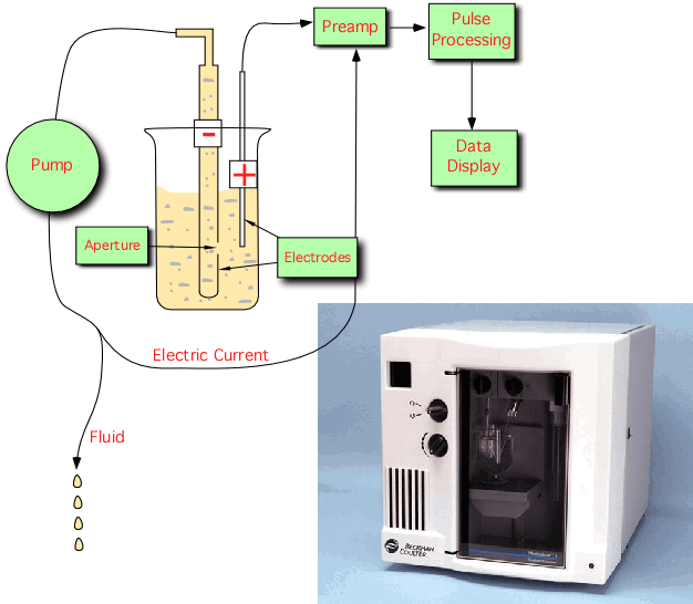
Figure 30.4. A coulter counter. Particle counters depend upon disruption of a current in a chamber. While there is an initial expense, they can save large amounts of time if many samples need to be counted. However, they cannot discriminate between microbes.
The advantage of this method is the simplicity of its operation and it reproducibility. As in microscopic counts, the machine cannot distinguish between living or dead cells or even between dust and bacteria. Any reasonably sized particle in the solution will be counted. There is also the expense of buying the counter, which can cost many thousands of dollars.
Viable counts
One of the most common methods of determining cell number is the viable plate count. Figure 30.5 shows a movie demonstrating the viable plate count. A sample to be counted is diluted in a solution that will not harm the microbe, yet does not support its growth (so they do not grow during the analysis). In most cases a volume of liquid (or a portion of solid) from the sample is first diluted 10-fold into buffer and mixed thoroughly. In most cases, a 0.1-1.0 ml portion of this first dilution is then diluted a further 10-fold, giving a total dilution of 100-fold. This process is repeated until a concentration that is estimated to be about 1000 cells per ml is reached. In the spread-plate technique some of the highest dilutions (lowest bacterial density) are then taken and spread with a sterile glass rod onto a solid medium that supports the growth of the microbe. It is important that the liquid spread onto the plate soaks into the agar. This prevents left over liquid on the surface from causing colonies to run together and the need for dry plates restricts the volume to 0.1 ml or less. A second method for counting viable bacteria is the pour plate technique, which consists of mixing a portion of the dilution with molten agar and pouring the mixture into a Petri plate. In either case are diluted so that individual cells are deposited on the agar and these give rise to colonies. By counting each colony, the total number of colony forming units (CFUs) on the plate is determined. By multiplying this count by the total dilution of the solution, it is possible to find the total number of CFUs in the original sample.
Figure 30.5. Viable Plate Count. Dilution plating and then spreading on an appropriate medium is a simple, yet effective way of determining the number of microbes in a sample. However, many microbes cannot grow in culture, so it does not give an accurate count of what is present in the environment.
One major disadvantage of the viable plate count is the assumption that each colony arises from one cell. In species where cells grow together in clusters, a gross underestimation of the true population results. One example of this is the genus Staphylococcus,, which is known to form clumps of microorganisms in solution. Each clump is therefore counted as one colony. This problem is why the term "CFUs per ml" is used instead of "bacteria per ml" for the results of such an analysis. It is a constant reminder that one colony does not equal one cell. Great care must also be taking during dilution and plating to avoid errors. Even one error in dilution can have large effects on the final numbers. The rate at which bacteria give rise to an observable colony can also vary. If too short an incubation time is used, some colonies may be missed. The temperature of incubation and medium conditions must also be optimized to achieve the largest colonies possible so that they are easily counted. Finally, this technique takes time. Depending on the organism, one day to several weeks might be necessary to determine the number of CFUs that were present when the experiment started. Such information may no longer be useful for many experiments.
Despite its shortcomings, the viable plate count is a popular method for determining cell number. The technique is sensitive and has the advantage of only counting living bacteria, which is often the important issue. Any concentration of microorganism can be easily counted, if the appropriate dilution is plated. It is even possible to concentrate a solution before counting, as is often done in water analysis, where bacterial populations w\are usually at low density. The equipment necessary for performing viable plate counts is readily available in any microbiology lab and is cheap in comparison to other methods. Finally, by using a selective medium it is possible to determine the number of bacteria of a certain class, even in mixed populations. These advantages have made viable plate counts a favorite of food, medical, aquatic and research laboratories for the routine determination of cell number.
Yet another method of determining the number of viable cells in a culture is called the most probable number method. By this method a culture is diluted to point where a certain small amount of that culture should contain approximately one cell, then multiple separate tubes of fresh culture medium are inoculated with aliquots of that small amount. After a suitable length of time, the tubes are checked to see how many of them display obvious bacterial growth. The fraction of tubes with growth then can be fitted to a curve to predict the actual number of viable cells in the starting culture, since the distribution of cells in the in the inoculated tubes must follow a Poisson distribution. Obviously, since we do not known exactly how much to dilute the culture before the samples are distributed into the tubes, several different dilutions must be tested. This way one of them will have a reasonable number of both "positive" and "negative" tubes. The precise nature of the curve fitting is more detailed than we need to review here, as is the statistical analysis that supports it.
Change in the amount of a cell component
In situations where determining the number of microorganisms is difficult or undesirable for other reasons, the use of indirect methods can be an excellent alternative. These methods measure some quantifiable cell property that increases as a direct result of microbial growth.
The simplest technique of this sort is to measure the weight of cells in a sample. Portions of a culture can be taken at particular intervals and centrifuged at high speed to sediment bacterial cells to the bottom of a vessel. The sedimented cells (called a cell pellet) are then washed to remove contaminating salt, and dried in an oven at 100-105 °C to remove all water, leaving only the mass of components that make up the population of cells. An increase in the dry weight of the cells correlates closely with cell growth. However, this method counts dead as well as living cells. There might also be conditions where the dry weight per cell changes over time or under different conditions. For example, some bacteria that excrete polysaccharides have a much higher dry weight per cell when growing on high sugar levels (when polysaccharides are produced) than on low. If the species under study forms large clumps of cells such as those that grow filamentously, dry weight is a better measurement of the cell population than is a viable plate count.
It is also possible to follow the change in the amount of a cellular component instead of the entire mass of the cell. This method may be chosen because determining dry weights is difficult or when the total weight of the cell is not giving an accurate picture of the number of individuals in a population. In this case, only one component of the cell is followed such as total protein or total DNA. This has some of the same advantages and disadvantages listed above for dry weight. Additionally, the measurement of a cellular component is more labor-intensive than previously mentioned methods since the component of interest has to be partially purified and then subjected to an analysis designed to measure the desired molecule. The assumption in choosing a single component such as DNA is that that component is relatively constant per cell. This assumption has a problem when growth rates are different because bacterial cells growing at high rates actually have more DNA per cell because of multiple initiations of replication.
Turbidity
A final widely used method for the determination of cell number is a turbidometric measurement or light scattering. Figure 30.6 shows an example of a spectrophotometer. This technique depends on the fact that as the number of cells in a solution increases, the solution becomes increasingly turbid (cloudy). The solution looks turbid because light passing through it is scattered by the microorganisms present and the turbidity is proportional to the number of microorganisms in the solution. The turbidity of a culture can be measured using a photometer or a spectrophotometer. The difference between these instruments is the type of light they pass through the sample. Photometers, such as the Klett-Summerson device, use a red, green or blue filter providing a broad spectrum of light. Spectrophotometers use prisms or diffraction gratings supplying a narrow band of wavelengths to the sample. Both instruments measure the amount of transmitted light, the light that makes it from the light source through the sample to the detector.
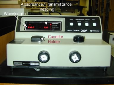
Figure 30.6. A Spec20D Spectrophotometer. A common, yet simple spectrophotometer made by Bausch and Lomb, the Spec 20D, is a reliable instrument for determining turbidity readings. After setting the wavelength and calibrating the machine, a sample is placed in the cuvette holder. The absorbance is read from the digital display.
When measuring light scattering it is important to consider the wavelength of light used a bacterial culture. Microorganisms may contain numerous macromolecules that absorb light, including DNA (254 µm), proteins (280 µm), cytochromes (400-500 µm), and possible cell pigments. When measuring bacteria by light scattering it is best to pick a wavelength where absorption is at a minimum and for most bacterial cultures wavelengths around 600 µm are a good choice. However, the exact wavelength chosen is species specific.
The amount of light transmitted through a sample is inversely proportional to cell number and can be expressed in the equation shown in Figure 30.7.
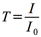
Figure 30.7. Transmittance. The relationship of transmittance to light entering and leaving the sample.
Where T is the light transmitted, I0 is the light entering the sample and I is the light passing through to the detector.
Due to the nature of light scattering, transmittance decreases geometrically as the cell numbers increase. It is more intuitive to think of the units increasing as growth increases and for most bacterial analysis, transmittance is converted into absorbance using the equation in Figure 30.8

Figure 30.8. The definition of absorbance. Absorbance is defined as the negative log of transmittance.
Absorbance increases in a linear fashion as the cell number increases. When measuring growth of a culture the term optical density (OD) is normally used to more correctly represent the light scattering that is occurring; under optimal conditions, little light is actually absorbed by the culture so the term absorbance is misleading.
For most unicellular organisms changes in OD are proportional to changes in cell number (within certain limits) and therefore can be used as a method to follow cell growth. If a precise cell number for a given OD is desired, a standard curve can be generated, where viable plate count or cell mass is plotted as a function of OD. It also wise to develop a standard curve to verify that the OD is actually an accurate portrayal of cell growth. After the standard curve is made, it is then possible to simply measure the OD of the culture and read the cell number from the curve.
The turbidity of a culture is dependent upon the shape and internal light-absorbing components of the microorganism and therefore turbidity readings are species-specific and cannot be compared between different microbes or even between different strains of the same species. As above, there are microbes that change cell size or shape at different stages of growth, which introduces some inaccuracy to this method of cell counting. Also both living and dead cells scatter light and are therefore counted. However, the method is very rapid and simple to perform and provides reliable results when used with care, so it is an extremely common method of real time analysis of prokaryotic populations. Turbidometric measurements also do not destroy the sample.
30 - 3 Visualizing microbes
Another important facet of microbiology is the observation of microbes and due to their small size, microscopes are necessary. Besides being able to visualize cell morphology and specialized structures, microscopes can even be used to identify bacteria in mixed samples when combined with certain fluorescent probes. These instruments are thus becoming indispensable tools in microbial ecology as well as their traditional use for observation and in identification.
Staining microbes
Before observing microorganisms, they must be placed on a suitable physical support so that they can be observed under a microscope. For light microscopes this simply entails placing a bit of culture on a glass slide. All liquid is allowed to evaporate and the microbes are then heat-fixed to the slide, usually by heating the slide momentarily over a Bunsen burner. Heat fixation breaks down some of the outer cell wall components, making them sticky, and cements the microbes to the slide so that they will not wash off during subsequent staining procedures. The slide is then cooled and ready for staining. Figure 30.9 shows the preparation of a smear.
Figure 30.9. Smear preparation. Before a sample can be stained, a sample must be applied to a slide and then heat-fixed to cement the cells to the slide.
Stains for the light microscope
In their natural state, many microorganisms are nearly transparent and not easily visible. They are made of water and other materials that do not readily absorb light and thus can be difficult to detect. A method is often necessary to differentiate microorganisms from the surrounding background and many staining techniques have been developed for this purpose. Figure 30.10 shows the structure of crystal violet.
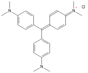
Figure 30.10. Crystal Violet. The structure of crystal violet. Note the positive charge that allows the dye to bind to the bacterial cell.
In most staining protocols a dye that readily absorbs light is mixed with a smear of microorganisms. The dyes contain charged groups and they readily bind to various macromolecules on the microbes. However, these dyes do not bind to the glass surface and are therefore easily washed from the background. After staining, one ends up with a smear where certain structural features of the microorganisms take on the color of the dye and the surrounding background is colorless. Stains have two important functional groups, the chromophore group and the auxochrome group. The chromophore group contains arrays of doubles bonds that absorb light and gives the stain its characteristic color. The auxochrome group contains either a positive or negative charge and allows the dye to bind microbial structures of opposite charge. The charge also makes the dye more soluble in aqueous medium, often a necessity for biological studies.
There are different stains that are used with different types of microscopes. Here we will introduce just a few examples to give you a general idea of the types of staining protocols. In a simple stain the smear is flooded with a single dye and allowed to incubate for a minute or two after which excess dye is rinsed off the slide. All microbial cells in the specimen that bind dye will be the same color. Simple stains can be positive stains, where the dye binds to the microbe and its structures, or negative stains, where the dye is repelled by the microbe, but stains the background. Note that in the latter case the stain is not washed off the slide. Figure 30.11 shows a simple stain with safranin and a negative stain, the capsule stain.
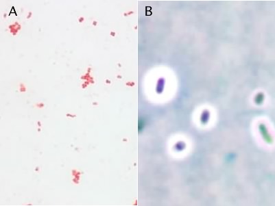
Figure 30.11. The simple stain and the capsule stain. Panel A is a photomicrograph of a simple stain of Staphylococcus epidermidis. Panel B shows an India ink stain (a negative stain) of Klebsiella planticola
In a differential stain, the smear is exposed to a series of different dyes. This technique takes advantage of the fact that particular structures have variable affinities for specific dyes. The first dye is applied to the smear and then a fixing reaction, either another chemical or heat, is applied so that those cells that have bound the dye retain it. A washing step removes any unbound dye and a second dye can be applied as a counter stain.
The Gram stain is the most commonly used differential staining procedure. Smears are first exposed to the dye crystal violet, which stains all bacterial cells purple. Crystal violet penetrates many bacterial structures, binding to the negative charges throughout the cell. Excess crystal violet is then washed off the cells and iodine is applied. Iodine reacts with the crystal violet forming complexes that become trapped in some cells. Subsequent treatment with alcohol-acetone decolorizes cells that do not bind the crystal violet-iodine complex tightly. Finally a counter stain with safranin, a red dye, stains all cells parts pink. The net effect is that all cells can be visualized by the red stain, yet Gram-positive cells can be recognized in the mix by their violet stain. Figure 30.12 shows the steps of the Gram stain
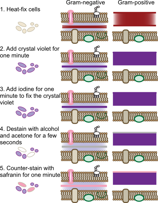
Figure 30.12. Steps of the Gram stain. The Gram stain is a four-step process that differentiates cells based upon their cell wall structure. The behavior of gram-positive and gram-negative cell wall is shown. Note that the dyes will also bind to any other negative-charged compounds in the cell, but only binding to the peptidoglycan is shown.
The Gram stain was originally developed by the Danish physician Hans Christian Gram in 1884 to differentiate pneumococci in samples of lung tissue. At the time the cellular basis of the stain was not clear, but we now know it depends upon the cell wall structure of the microorganism. For microbes of the domain Bacteria, cells containing thick peptidoglycan layers are able to retain the crystal violet-iodine complex and appear Gram positive. Those that have thinner peptidoglycan layers are easily decolorized by the alcohol wash and are only visible after counter-staining, thus being Gram negative. The staining procedure of Gram was actually differentiating the two basic cell wall structures present in the Bacteria. As discussed in Chapter 3, there are some cells that contain a Gram-negative cell wall structure that stains Gram positive due to other properties, and the opposite is also true. The archaea have very different cell wall structures and the Gram reaction of each species does not normally predict anything useful about its cell wall.
Another important stain is the acid-fast stain. During his work on the causative agent of tuberculosis, Robert Koch had a difficult time visualizing the bacteria. The microbes would not bind conventional stains and it was difficult to detect them in the sputum of infected patients. After much experimentation, he settled on the acid-fast stain developed by Paul Erhlich and the microbes became visible. In the acid-fast stain, the smear is initially stained by heating cells to near boiling in a solution of the stain carbol fuchsin and then destaining with acid-alcohol. The destaining decolorizes non-acid-fast bacteria and these are then counterstained with methylene blue. Acid-fast bacteria appear red under the microscope, while non-acid-fast bacteria are blue. Figure 30.13 shows the acid fast stain.
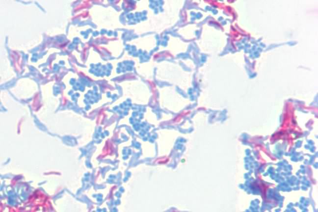
Figure 30.13. The acid-fast stain. A photomicrograph of Mycobacterium smegmatis (pink) and Micrococcus luteus (blue) at 1000x magnification. M. smegmatis is acid-fast, retaining the carbol fuchsin dye, thus appearing pink. M. luteus is not acid-fast, loses the carbol fuchsin during decolorizaiton, and is counter-stained with methylene blue.
Acid-fast staining is crucial in the diagnosis of tuberculosis, which is caused in humans by Mycobacterium tuberculosis and related species. These microorganisms and a number of others have very hydrophobic, waxy cell walls that repel most stains, but the acid-fast procedure causes the carbol fuchsin dye to penetrate the walls and is trapped within the wall upon cooling.
It is also possible to stain specific structures in microorganisms and we call these structural stains. A good example of a structural stain is the endospore stain. Endospores have tight compact cell walls that are impermeable to most dyes and in the Gram stain they appear as colorless regions inside of the cell. In the endospore stain, the cells are boiled in the presence of the dye malachite green. The higher temperature causes the spore coat to expand, allowing the dye to penetrate the spore and malachite green is trapped inside the spore upon cooling. A wash with water removes the dye from vegetative cells and these are then counterstained with safranin. When examined using a microscope, spores appear green and vegetative cells are pink. Structural stains to detect flagellum, phosphorus globules and various other inclusions inside of cells are also common. Figure 30.14 shows an example of at structural stain, the endospore stain.
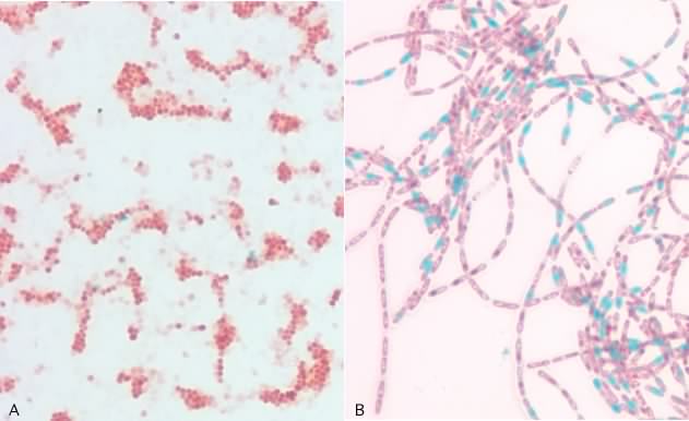
Figure 30.14. The endospore stain. A photomicrograph of an enodspore stain. Spores present in the picture stain green, while the vegetative cells stain red. A) Staphylococcus epdiermidis which does not form endospores. B) The endospore-forming rod, Bacillus cereus.
Most of the staining protocols we have talked about here were developed at the dawn of microbiology more than 100 years ago. The advent of 16S rRNA sequencing and phylogenetic analysis had lead to the development of a new set of tools that have similarities to staining protocols. Literally thousands of 16S rRNA sequences are known and analysis of these pieces of nucleic acid have lead to the discovery of regions that are diagnostic of specific species, families of microorganism or entire domains. It is therefore possible to design nucleic acid probes that bind to only a particular species, genera, family or an entire domain of microorganisms. This works because stable binding of two nucleic acid sequences depends on exactly how similar the two sequences are. The hybridization conditions (for example, the temperature and level of salt) can therefore be chosen so that only organisms with the desired sequences hybridize to the probe efficiently (for more detail see "DNA arrays" later in this chapter).
This in itself is interesting, but it becomes even more powerful when these probes are attached to fluorescent dyes that emit a specific color when exposed to UV light. A microbial sample is fixed to a surface in such a way that the nucleic acid and proteins stick, but the cells are permeable. To this is added a fluorescently tagged DNA probe and it is allowed to incubate for a period of time. Under appropriate conditions the probe penetrates the microbes and binds only to those bacteria that contain a matching 16S rRNA sequence. The poorly hybridizing probes are removed by an appropriate wash. When examined under a fluorescence microscope (see below) only microorganisms of the desired target group fluoresce. This provides a powerful new tool to access what is present in any environment. Figure 30.15 shows an example of a fluorescent stain.
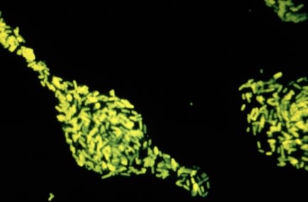
Figure 30.15. A fluorescent stain. A fluorescent dye is attached to antibodies against Salmonella enterica. When these antibiodies are mixed with a test smear, if S. enterica is present the antibody will attach and glow brighting in a fluorescent microscope. In this way it is very easy to test for the presence of a microbe of interest.
Staining for the electron microscope
Preparation of samples for the electron microscope is more complex than for the light microscope and a detailed description of it is beyond the scope of this book. There are also two different types of electron microscope, scanning and transmission, and the sample preparation for each of them is somewhat different. However, a few general points are worth mentioning. The resolution of the electron microscope is much higher than that of the light microscope, so the goal here is not to see microbes but rather to see specific structures and even molecules within microbes. However, this requires that these structures scatter electrons, something that they normally do not do to any great extent because they are largely composed of small atoms (C, H, N and O). To create more scattering, these stained with atoms of heavy metals such as osmium, lead or uranium. As with stains for light microscopy, the stains themselves fall into two general categories. Negative stains employ salts of these metals that fail to bind to most biological structures, so that the absence of staining indicates the presence of a structure. Positive strains employ salts that tend to bind to those same structures. This staining is performed on samples that have been desiccated and fixed in some way. Finally, because the electrons must pass through the sample, the support must be transparent to electrons. This is accomplished by using thin support films such as nitrocellulose, which is placed on a small copper grid to give it some stability - the regions of the sample in the holes of the copper grid are what is analyzed.
To view external structures, whole microbes are fixed, stained and then observed. It is also possible through various treatments to section cells, either by slicing on an ultramicrotome, an instrument that can create thin sections through a microbe of less than 100 nm, or by freeze fracturing microbes. Freeze fracture is a method in which frozen samples are sheared and then strained. It turns out that the plane of shearing often occurs along interesting structures, such as between bipolar membranes. The result is an image of the actual membrane surface showing specific proteins.
Microscopes
Magnification and resolution
A microscope enlarges the size of the intended image so that it is visible to the scientist. Most modern microscopes have two or more lenses and are therefore called compound microscopes. The lenses serve as prisms and bend light to a focal point and the distance from the lens to the focal point is called the focal length. Our eyes have a focal length of about 25 cm and cannot resolve objects by moving any closer. The focal length limits the smallest object we can see to about 0.2 mm in size. Convex lenses, those that are thick in the middle and narrower at the ends, shorten the focal length and when brought between an object and observer cause the object to appear much larger. If machined carefully a single lens can magnify an object up to several hundred times. However, if two lenses are placed one after another between object and observer, their magnification strength is multiplied. Thus if a 100X lens and a 10X lens are used, the total magnification would be 1000-fold.
Magnification is necessary to see very small objects, but the resolving power of the microscope (or the resolution of the object) is of equal importance. Resolution is defined as the ability to separate or distinguish objects that are close together and can be described by the equation in Figure 30.16
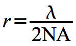
Figure 30.16. The resolution equation. A listing of the parameters that influence the resolution of a microscope. The resolution of a microscope is mostly limited by the wavelength used to visualize the sample. Light microscopes have as a maximum resolving power of 200 nm.
Where r is the resolution, λ is the wavelength of light, and NA is the numerical aperture of the lens.
For good microscopy it is desirable to have the resolution be as small as possible. This equation implies that it should be possible to improve resolution by either increasing the numerical aperture or by decreasing λ. In practice the numerical aperture of a lens is set by the construction of the lens and does not change. This leaves λ as a useful variable, and by decreasing the wavelength of light it is possible to increase the resolution. The resolution of the average 100 x objective lens (NA ~ 1.25) using short wavelength light (360 nm) is about 0.19 µmeters. If a longer wavelength of light is used (700 nm) the resolution increases to 0.39 µmeters.
Light microscopes
Many types of light microscopes have been developed over the years and they vary in price, sophistication and purpose. The simplest microscope is the light microscope that is basically a tube containing lenses and prisms that can magnify a sample to about 1000-fold. For magnification of greater than 100x, oil immersion lenses are used, which involves filling the small volume between the glass cover slip covering the sample and the microscope lens with oil. The refractive index of this oil is almost the same as that of glass, which thus avoids the problem of the light being bent through multiple environments and assists in the resolution as described by the equation in the previous section. Because of the general transparency of living samples, stained specimens are necessary and these procedures kill the bacteria. Objects in light microscopes appear dark in a bright background. Figure 30.17 shows an example of a typical light microscope.
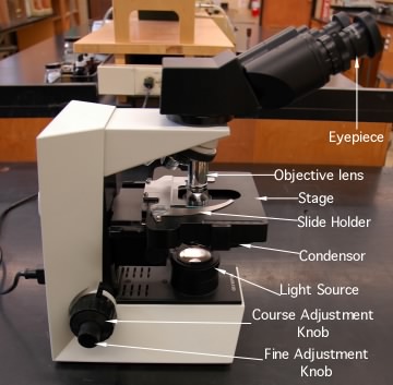
Figure 30.17. The light microscope. Pictured are the light microscopes used in the teaching labs of the Bacteriology Department at the University of Wisconsin-Madison. The various parts of the microscope are listed.
While light microscopes are valuable, it is sometimes desirable to view living microorganisms, for example to observe their chemotactic behavior. A phase contrast microscope is an excellent tool for these types of observations. A phase contrast scope depends upon the fact that light passing through a bacterium is slightly refracted and its phase is retarded 1/4 wavelength. The phase of light refers to positioning of the valleys and crests of the light waves in relation to one another. When light is in phase the light waves valleys and crests coincide, Figure 30.18, and when it is out of phase, they do not. If a sample contains bacteria, the light passing through the microbes will be shifted in comparison to light that did not hit any microbes. However our eyes are unable to detect slight phase differences.
Figure 30.18. Waves and phases. Wave B is one-quarter wavelength out of phase with wave A. Wave C is one-half wavelength out of phase with wave A. If wave A and wave C collide, they will cancel each other out.
In phase microscopy, an optical trick is used to increase the contrast between the cells and their environment by artificially increasing the difference between light that has passed through the microorganism and light that has not. Three basic modifications are made to the phase scope to make this trick work: 1) uniformly in-phase light is used to illuminate the sample; 2) an annular diaphragm, located inside the condensor, permits only a ring of light to pass through the sample and into the objective; and 3) a phase-shifting plate, which is located inside each phase-contrast objective, contains a ring of material that advances the phase of the light 1/4 wavelength. The ring of light from the annular diaphragm is focused on the sample by the condensor. Light then passes through the sample, into the objective lens and up to the eye. To understand how the phase microscope works, imagine two sets of light rays that are passing through a slide on the microscope stage. The great majority of light rays pass through the sample, but are not altered by any microorganisms. The optics of the microscope are set up so that unaltered light rays coming from the sample pass through the phase-shifting material in the phase plate and are advanced 1/4 wavelength. A subset of light rays passing through bacteria have their phase retarded 1/4 wavelength, and are refracted. This slight refraction causes these light rays to miss the phase-shifting material in the phase plate, but they are still collected by the objective lens. As the two sets of light rays now journey towards the eye, they are focused and magnified by lenses in the eyepiece for viewing. The light rays that passed through the sample and contacted bacteria are now 1/2 wavelength out of phase with the light rays that did not. When light rays 1/2 out of phase mix together, they cancel each other out. Thus, a portion of the light coming from the background that did not pass through a microorganism will cancel out any light ray that did pass through a microbe and the object will appear dark to the viewer. Microorganisms typically appear dark in a light background and are called phase dark. Some objects that do not allow light to pass through them, such as bacterial endospores, appear very bright in the microscope and are termed phase-bright. Figure 30.36 shows an example of a phase contrast microscope image.
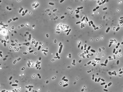
Figure 30.36. A phase contrast image. A phase contrast image of an Azotobacter sp. isolate at 100x magnification. This microbe was enriched from soil using Burk's medium.
Dark-field microscopes direct light at a sample from the side. Light hitting objects in the specimen is scattered in all directions and some of it is collected by the objective lens and directed to the eye. In dark-field microscopy, microbes appear light in a dark background. These microscopes have a higher resolving power than other light microscopes and are useful for examining objects with small diameters. Small or thin bacteria such as the spirochetes are only easily detected using dark-field microscopes and this can make them invaluable for studying such bacteria. Dark-field microscopes can also be used to visualize flagella or flagellar tufts in some species of microorganisms. Figure 30.19 shows an example of a specimen viewed through a dark-field microscope.
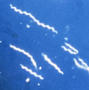
Figure 30.19. Dark-field micrsocopy. Visualization of Borrelia burgdorferi as seen through a dark-field microscope. B. burgdorferi is a very thin, spirillum and is difficult to visualize with a normal light microscope.
Another type of light microscope is the fluorescence microscope. This scope depends upon the ability of certain organic compounds to fluoresce. That is the ability of a molecule to absorb light at one wavelength and release it at another. Thus if a specific wavelength of light illuminates a sample, the fluorescent compound absorbs it and releases a second, distinctive wavelength that is easily visible using these microscopes. Fluorescent microscopes contain filters on their light sources that only allow a desired wavelength to illuminate the sample. As in the case of the dark-field microscope, light enters the sample in a direction perpendicular to the path it must travel to reach the objective and the observer. Therefore, the observer only sees the re-emitted fluorescent light. There are many fluorescent compounds that can be detected and microbes containing them fluoresce a distinctive color. For example, chlorophyll is naturally fluorescent and cyanobacteria fluoresce red when light of 546 nm illuminates them. Other microbes that contain no natural fluorescent compounds can be stained with fluorescent dyes, such as acridine orange. As we mentioned earlier, specific DNA probes attached to fluorescent dyes can also be used to identify specific groups of microorganisms.
Specialized microscopes
There are two major limitations to light microscopy. First, all forms of light microscopy end up displaying a two-dimensional image of a three-dimensional sample. Second, the use of light to illuminate the sample limits the maximum achievable resolution. Recall that the equation for resolution contains in its numerator the wavelength of electromagnetic radiation hitting the sample. The smallest wavelengths of visible light are in the blue spectrum and wavelengths below this are not visible to our eyes. Therefore while it is possible to make compound light microscopes that magnify samples many thousands of times, they are limited by the resolution that visible light can achieve to about 1,000-fold.
There are two main approaches to improving the visibility of samples beyond what a conventional light microscope can achieve. One method involves the use of special sensors or light sources. An example of this is the differential interference contrast microscope. This microscope employs a polarizer that creates planar polarized light. This is light that is all in one plane and entirely in phase. This light is split into two beams and both are directed at the sample, see Figure 30.20. Microbes in the sample have a slightly different refractive index than the surrounding environment and they cause a subtle change in the phase of the impacting rays. When the beams are recombined, the light waves that passed through objects in the sample will be slightly out of phase and an interference pattern will be established, which intensifies subtle differences in refractive index around cellular structures. The largest effect is around the edges of features that have distinct borders, thus differential interference contrast microscopy enhances the appearance of nuclei, spores, vacuoles and other inclusions.
Figure 30.20. Differential interference contrast microscopy. A movie of the developmental cycle of Caenorhabditis elegans, a nematode, is shown. C. elegans is heavily studied as a model system for development in eukaryotes. Beginning with a fertilized egg, scientists have tracked the developmental fate of all cells in the nematode all the way to the adult stage, containing over 900 cells.
A second example of using a specialized light source is scanning confocal microscopy. This is a type of fluorescence microscopy where a sample is illuminated with one wavelength that is absorbed by the sample. The excess light energy is later released as longer wavelength light and this is then collected and observed. Images generated by conventional fluorescence microscopy are degraded by the collection of light that is out of the focal plane. In scanning confocal microscopy this problem is solved by illuminating a single spot on the sample and scanning across the sample to collect a complete image. The spot of light is generated by passing light through an aperture or more commonly by using a laser of appropriate wavelength. This method avoids out-of-focus light collection because only a single focused spot is illuminated at any one time, and light intensity drops off rapidly above and below the focal plane. Confocal microscopes when operated in ideal situations can achieve resolutions that are 1.4 times higher than with a conventional light microscope. Figure 30.21 shows an example of a scanning confocal microscope.
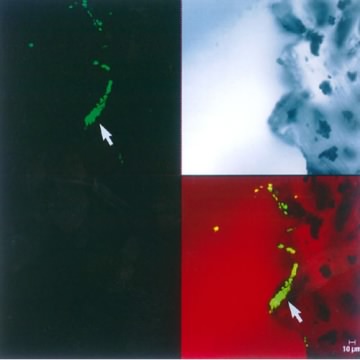
Figure 30.21. An image from a scanning confocal microscope. The upper left image shows a section from the tip of shunt tubing stained with SYTOX Green nucleic acid stain and examined by scanning confocal microscopy. The shunt was from an patient who had an infection with Coccidioides immitis that did not respond to treatment. The fungus had formed a biofilm on the shunt and prescribed antifungals could not penetrate the biofilm. The upper right image shows an unstained, transmitted light microscopic image of the same area of the edge of the tubing. The bottom right image shows a recombined image with the nucleic acid stain colocalized with the transmitted light image. The recombined image shows that a substantial (~30 µm) biofilm composed of 4- to 6-µm cells has colonized the scalloped surface of this tubing. (x630 total magnification mosaic). Image used from Larry E. Davis, Guy Cook, and J. William Costerton. Biofilm on Ventriculo-Peritoneal Shunt Tubing as a Cause of Treatment Failure in Coccidioidal Meningitis. Emerg Infect Dis [serial on the Internet]. 2002 April
Another example of a powerful method for visualizing cells is the atomic force microscope, which does not involve light at all and is not exactly a microscope in most senses of the term. It involves an almost unbelievable technology in which a tiny stylus is moved within a few atom lengths of the sample. This allows the detection of weak repulsive atomic forces between the stylus and molecules in the sample. As the stylus scans across the sample, changes in topology, due to objects such as individual atoms and molecules present in the specimen, cause the stylus to rise and fall. A computer collects this data and by combining the results of a complete scan an image can be created. Image resolution of the atomic force microscope can be incredibly small, magnifying samples up to 1,000,000 times, allowing the resolution of individual large metal atoms. It also has the advantage of simple sample preparation in comparison to the electron microscope. However, these microscopes are obviously expensive and take a long time to generate an image. Its extreme resolution also means that it is useful only for very small structures present on a very flat surface. This means that it is useful for examining individual protein molecules on an artificial surface, but not so successful in examining the uneven surfaces of real biological samples. Figure 30.22 shows an example of an AFM microscope.
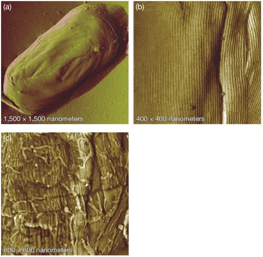
Figure 30.22. Endospores visualized with atomic force microscopy (AFM). AFM allows visualization of specimens at incredible resolutions. Picture here is an endospore from Bacillus atrophaeus at progressively higher magnifications. High magnification in (b) reveals an array of rod-like structures. Image courtesy of Lawrence Livermore National Laboratory
Electron microscopes
One method of increasing the resolution of a microscope is by using electromagnetic waves of a shorter wavelength than visible light. Waves outside of the visible spectrum are of course not visible to the naked eye and detectors have to be used to convert the output of these scopes into something that we can see. A convenient choice for this type of work is the electron. While most students think of electrons as particles, remember the dual particle-wave properties of elementary particles such as the electron and the photon. Electrons can be treated as waves, having characteristic wavelengths and can also be focused just like visible light, but with a magnetic lens instead of a glass one. The wavelength of electrons is much shorter that of light and thus can magnify things up to 100,000-fold. Indeed, the best pictures with these machines can resolve single atoms, albeit of heavy elements such as gold. This enables visualization of structures down to the size of individual protein molecules. However, electron beams are dispersed by particles in air and specimens therefore must be examined in a vacuum. As mentioned earlier, most biological samples do not scatter electrons well and have to be stained with heavy metals such as gold, osmic acid, permanganate, uranium or lanthanum salts. Treatment with these types of stains can distort microbial structures, as can the dehydration of samples in a vacuum.
There are two general methods of electron microscopy: transmission electron microscopy (TEM) and scanning electron microscopy (SEM). In TEM the set up of the microscope is analogous to that for a light microscope where the beam of electrons pass through the sample and is focused and collected on the other side for observation, Figure 30.23. Electrons cannot penetrate very far into tissues and samples must be very thin. A microbial sample is typically sliced into many sections and these are view in series to get a picture of the entire organism. If the outside structures of a microorganism, such as its flagella or pili, need to be observed, a negative staining technique allows observation by TEM. These pictures tend to be analogous to that obtained with a light microscope, except that the resolution is much higher.
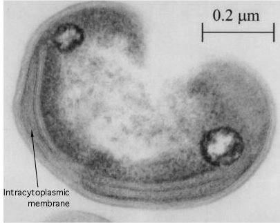
Figure 30.23. A transmission electron micrograph. A thin section of a Methylocystis sp, isolated from a rice patty.
There is another little complication here in that you are detecting structures by their ability to absorb electrons. But electrons moving at high speed have a lot of energy, so their absorption actually damages the delicate structures we want to resolve in the sample. The highest resolution pictures then can only be observed for a limited amount of time. This raises a common philosophical point that we often ignore. The methods we use to examine the behavior of microbes and the parts within them often perturb the very thing we wish to analyze. This is true of genetic approaches as well as biochemical ones. There is really no way around this problem except to be aware that we are doing it.
Alternatively, SEM, Figure 30.24, can be used to create a more 3-dimensional image of a sample. A sample is first coated with a thin film of heavy metal atoms so that it will absorb electrons that impact its surface. An electron beam then scans across a sample much as the electron gun in a cathode ray tube (found in older televisions and computer monitors) scans across the screen. The sample is set up so that the electrons striking the metal atoms on the target cause the emission of a shower of secondary electrons that is seen by a collector. The number of electrons that reach the collector is dependent upon the angle of the cell surface relative to the collector. By measuring the number of electrons that bounce off each spot of the specimen it is possible to create an image of the sample. As you might guess from this description, detecting scattering means that SEM has much poorer resolution than TEM. However, it provides stunning views of cells and their larger constituents that have a curious three-dimensional feel.
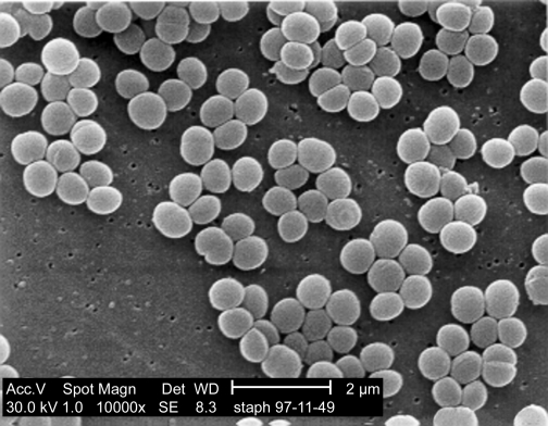
Figure 30.24. A scanning electron micrograph. An SEM of Staphylococcus aureus. Note the three dimensional appearance of the image.
X-ray crystallography
X-ray crystallography is also not microscopy, but it does provide images of molecules and involves variations on some of the same themes of microscopy, so we will handle it in this section. The actual methods of X-ray crystallography are not appropriate for this text, but a general description should be helpful. Scientists take highly purified proteins and create very concentrated solutions of these. They then let these sit under a variety of conditions and see if any small crystals form, rather like you might grow crystals of sugar on a piece of string suspended in a concentrated sugar solution. When crystals are found - and sometimes it is very difficult to obtain nice crystals of a reasonable size - they are removed and placed in a machine that shines X-rays on them. Consistent patterns in the crystal, formed because all of the proteins have lined up in the same way, diffract (essentially the same as reflect) the X-rays to specific positions. The scientists then examine all of the places to which the X-rays have been diffracted and, though some very complex mathematical analysis, are able to compute the two-dimensional electron density map at a given plane in the sample. These two-dimensional maps are then stacked together to reveal a three-dimensional density. However, this image of the overall electron density does not exactly reveal the actual bonds of the molecule in the sample. For that, the known sequence information (in the case of a protein) is carefully lined up ("threaded") with that electron density in such a way that it makes consistent sense. Then a structure can be modeled from this and statistically refined. The final product is a three-dimensional image of the positions of most or all of the atoms of the molecule, depending on the resolution of the analysis. Very high quality crystals can allow a resolution of less than 2 angstroms, which effectively means that one can visualize the positions of all atoms in the molecule larger than hydrogen. Some extremely high-resolution images can even resolve individual hydrogen atoms. Figure 30.25 shows examples of the models of a protein at different resolutions.
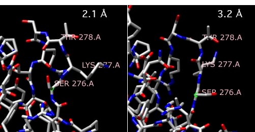
Figure 30.25. Comparing X-ray resolutions. Two structures of alpha amylase II from Thermoactinomyces vulgaris R-47. One structure is at 2.1 Å, while the other is at 3.2 Å Note that the structure of the three highlighted amino acids, serine 276, lysine 277 and threonine 278 changes as the resolution gets higher and more accurate.
So what does this really tell us? It reveals the exact structure of the form of the protein that crystallized in three dimensions. It also provides a good guess about one of the forms of the protein in solution, but there is always the chance that the crystallization itself perturbed the structure a bit. However, even if the determined structure does represent a structure that exists in solution, you should remember that proteins are almost always flexible molecules. Indeed, it is essential for enzymes to change shape a bit when they bind their substrates and again when the release that substrate. Some proteins actually undergo very large structural changes during the performance of their roles in the cell. As a consequence, a single structure of a protein represents no more than one possible form assumed by the protein in the cell. On the other hand, having any structure of a protein is essential if you are to understand physically how it performs its functions.
As the structures of more proteins are determined, we are getting a bit better at guessing the rules by which a protein's sequence determines its structure. At some point we will presumably not need to actually solve new protein structures, because our prediction methods will be so good, but that is a long time in the future. However, scientists have taken the first steps down this long road. Scientists have correctly predicted the 3-D structure of some small proteins (~20 residues) using only the primary sequence and a computer, but these were exceptional cases and accurate prediction of the structures of most proteins even of this size is currently beyond our abilities. However, there is another route to structure prediction whose application is already underway. Remember that evolution works by altering the function of existing proteins, and therefore one can make a reasonable prediction about a protein's structure if the structure of a homologous protein has been solved. Because completely novel protein structures are being solved at the rate a several per day, it is already the case that most newly sequenced genes can be roughly modeled for structure based on the known structure of a homologous protein.
30 - 4 Molecular techniques
Many modern techniques for detecting the presence of microorganisms and determining the sequence of their DNA depend on molecular biology techniques that first began to appear in the middle of the 1970's. In this section we give a somewhat detailed explanation of common methodologies that were used in part to generate much of the information we have talked about throughout this textbook. Of course the techniques talked about here are not comprehensive, but they do cover some of the more common (and oft mentioned) procedures of microbial molecular biology in use today.
Gel electophoresis
It is often very useful to separate different types of biological molecules so we can detect, analyze or even isolate them. When molecules with a charge are placed in an electric field and a current is applied, they move. One could therefore put electrodes on opposite sides of a beaker full of cell extract and the positively charged molecules would move to the negative electrode and negatively charged molecules would move to the positive electrode. This would not be very useful, because you could not easily tell where any molecules were in that solution nor could easily remove them without mixing. Molecular biologists therefore create electric fields in semi-solid material called gels. These can be made from a variety of things, from seaweed extract (agar and agarose) to chemically synthesized systems (acrylamide), but they have some similar properties. In all cases, they are loose structures that are full of water, but they differ in how dense the structures are. In other words, the size of the holes through the material can vary. If one creates a gel Figure 28.26, puts opposite electrodes at each end and puts some cell material in a little well in the center, the different molecules will migrate toward one electrode or another when the current is turned on. The rate at which they migrate will depend on their size and charge. Very charged molecules are strongly attracted to one electrode and move faster (all other things being equal) than less charged molecules. However, the molecules also need to wiggle through the holes in the gel, so small molecules move faster than larger ones (again, if all other factors are equal). Remarkably, the speed of migration is highly reproducible, so that all fragments of the same size and charge migrate at the same rate within a few percent.
Figure 30.26. An agarose gel. Pictured here is an agarose gel before it is run. Note the lanes at the top of the gel where sample can be loaded.
A critical feature of gels is that, unlike the case with the beaker above, when one turns off the current, the molecules not only stop moving, but one can find out where they are because they are fairly well trapped in the gel. Gels can even be dried down and saved. You can also determine the positions of specific molecules identified by various methods. But how do you know where these molecules are in the gel? There are several different approaches, depending on the nature of the molecules that are in the gel. Nucleic acids can be detected by stains that bind to only the nucleic acid and not to the gel, or by using radioactively labeled nucleic acid and then exposing the dried gel to film, which is exposed near the radioactivity (termed autoradiography). For proteins, detection of all proteins in the gel can also be performed with general stains or radioactive labeling.
It is even possible to detect a specific protein or a specfic nucleic acid in a gel and we will describe these methods in greater detail below.
Restriction Enzymes
Restriction enzymes evolved in many species of prokaryotes as a mechanism to protect themselves from foreign DNA that might enter the cell (see T4 in Chapter 13). Some of this foreign DNA might be that of bacterial viruses, but there are other sorts of selfish DNA molecules that a cell might want to protect itself from. The typical solution was an enzyme that would recognize a specific DNA sequence, typically 4 or 6 base pairs in length, and then cut both DNA strands whenever that sequence was found. Such a double-strand break destroys the ability of most DNA molecules to replicate and therefore would protect the host cell from entering DNA molecules. But how does the cell prevent its restriction enzyme from cutting the same sequences in its own DNA? The solution is that cells produce an enzyme that methylates the identical DNA sequence on both DNA strands, so that the restriction enzyme fails to recognize and cut it. So why doesn't the methylation system also protect the foreign DNA? That is because the foreign DNA will enter the cell in an unmethylated form, which is a very good substrate for the restriction enzyme and a poor one for the methylase. In other words, in most cases the restriction enzyme gets to the foreign DNA first, before the methylase can modify it. But that brings up yet another question: concerning that host DNA, how does the methylase beat the restriction enzyme? In this case the host DNA is normally methylated on both strands, but after replication, only the old strand is methylated. This hemi-methylated site is a very good substrate for the methylase (so the site is quickly converted to a fully methylated form), but is a terrible substrate for the restriction enzyme.
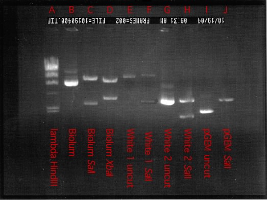
Figure 30.27. A finished agarose gel. Various plasmids isolated as part of a cloning experiment were run out on an agarose gel. (lambda HindIII) phage lambda DNA digested with the restriction enzyme HindIII. (A) the plasmid pGEM3Z from Promega corporation with the bioluminescent genes from Vibro fischeri cloned into it. (B) Plasmid in A digested with SalI. Note that he insert is digested out of the plasmid and is about 10 kB long. (C) Plasmid in A digested with XbaI. In this case the insert has an XbaI site and is cut. The plasmid also has one XbaI site. (D). (E-H) Various cloned inserts from Vibrio fischer. (I) plasmid pGEM3Z. (J) plasmid pGEM3Z cut with SalI.
Our use of restriction enzymes has little to do with their biology. As you might guess, if different organisms are going to use these systems for identifying foreign DNA, then each species needs to have different restriction enzyme target sites than most other organisms. As a consequence, there are a large number such enzymes, typically from different prokaryotic species, that have completely different target sequence. Companies over-express and purify these different enzymes of known target sequence and sell them, allowing the experimenter to cut their DNA at a variety of specific sequences. This is valuable in itself, since it can give you a lot of DNA of precise size and you can, for example, cut a plasmid preparation and run the fragments on an agarose gel, Figure 28-27, and isolate a particular DNA fragment. However the greatest utility of these enzymes has come from another property; they typically make staggered cuts at the site. This staggering means that there will be a 1-4 nucleotide region of single stranded DNA at every newly created end. Moreover, the single-stranded region of one end will be able to base-pair with the single-stranded region of any other DNA end produced by the same enzyme. This base pairing of a few bases is not strong, but it is good enough to allow DNA ligase, an enzyme that seals nicks in DNA, to fix both nicks and form a normal piece of double-stranded DNA. This has been critical for much of molecular biology because it allowed the scientist to cut-and-paste different DNA fragments together in a precise way. The increased use of PCR has made some of the uses of restriction enzymes obsolete, since PCR can be used to fuse any two sequences together and does not depend on the existence of specific sequences at desired positions (see below).
The restriction enzymes referred to above are ones that have relatively small recognition sequences of 4-6 bp, so the number of sites with such a sequence is fairly large in a piece of DNA as large as a chromosome. However, there are some enzyme that recognize longer sequences (8 bp) and probability dictates that such sequences are extremely rare. As a consequence, cutting an entire chromosome with such enzymes often gives a few to a few dozen discrete bands. These very large fragments can be very useful in trying to organize DNA sequence data (see below) into a pattern that represents the circular chromosome.
Cloning
Cloning has a variety of meanings that are only distantly related. In general, it means to produce many identical copies of something. For a prokaryotic molecular biologist, cloning has meant the ability to produce large amounts of a single DNA sequence. For a number of years, this was accomplished by using restriction enzymes to move the desired piece of DNA onto a vector like a plasmid or the genome of a bacteriophage. In each case, one can grow up cells with many copies of the vector, isolate the plasmid or phage, and then remove the desired piece of DNA from the vector using restriction enzymes. The different fragments were separated from each other on a gel. It was thus possible to make as many copies of the DNA as needed for experiments and one would then have cloned that specific DNA sequence. This process is diagrammed in Figure 28.28. Today, one typically obtains large amounts of a specific sequence more directly by PCR, which can amplify large amounts of DNA defined by the choice of two DNA primers.
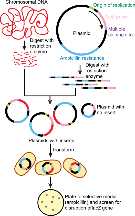
Figure 30.28. Cloning of target DNA. In the classic method of cloning, often called shot-gun cloning, purified target DNA is digested with the same restriction enzyme as a plasmid that will carry the DNA. They are then mixed together and the overhang of bases, created by the restriction enzyme digestion, hybridize. These newly formed plasmids, containing target DNA, are covalently closed using DNA ligase and transformed into a suitable host. Since transformation is an infrequent even, the plasmid is then selected for on solid medium containing a drug resistance the plasmid carries. In this case ampicillin.
As you might know from newspaper and movies, however, cloning has a rather different meaning: the production of multiple copies of an identical animal. Typically this is done by teasing apart the few cells of an early-stage fertilized egg, and then using each of these to create new and genetically identical individuals. Alternatively, cell nuclei can be extracted from certain cells of an adult animal and put in an environment (an egg) where again they can develop to a new organism. While there are certainly a number of ethical issues involved in this, particularly in the case of humans, you'll realize that this is roughly what prokaryotes do all the time.
Transformation
Transformation is the method that allows the introduction of bare DNA into a cell and naturally occurring transformation was covered in Chapter 12. Transformation has two hurdles to overcome: first, the DNA must be purified and this can be either plasmid or chromosome, linear or circular; and second, competent cells must be generated. Competent cells are those that can accept DNA. In the case of E. coli, there are a variety of recipes for performing this, but typically they involve multivalent cations and some time of incubation at low temperature, whereupon, a fraction of the cells (fewer than 10%) become competent to take up DNA. Somehow the process leads to the formation of dozens of "channels" per cell that can take up DNA. A number of other gram-negative bacteria have been successfully transformed with variations on this approach.
Gram-positive bacteria have to be treated differently, because of the differences in their cell wall. They can be incubated with degradative enzymes to remove the peptidoglycan layer and thus form protoplasts. When these latter cell forms are incubated with DNA and polyethylene glycol, one obtains cell fusion and concomitant DNA uptake. In both of these examples, if the DNA is linear, it tends to be very sensitive to nucleases so that transformation is most efficient when it involves the use of covalently closed circular DNA. Alternatively, nuclease-deficient cells can be used to improve transformation.
Finally, the technique of electroporation is becoming commonly used with bacteria. It essentially involves creating transient pores in the cells using electric current and can be used for both cell fusion and incorporation of DNA. When optimized for a particular organism, electroporation seems to be good for at least an order of magnitude increase in the frequency of transformants when compared to optimized transformation methods and in some species is the only efficient way of getting DNA into cells.
DNA Sequencing
DNA sequencing has gone through huge changes in the past 30 years. In the late 1960's it took a graduate student 4 years to sequence 12 bases that form the sticky ends of phage lambda and now millions of bases are sequenced daily around the world. Continuous innovation keeps changing the details of the way DNA is sequenced, but the method is still based on the idea of running reactions that distinguish the four different types of bases and causing random errors in the process so that an entire spectrum of different sized fragments is created.
Currently, most sequencing reactions rely on synthesis of DNA using DNA polymerase from thermophilic organisms. In a manner similar to PCR, the reaction contains a template to be sequenced, a primer and the four nucleoside triphosphates. Note however, that there is only one primer, not two as in PCR. To this reaction is also added a small amount of the four nucleoside triphosphates where the 3'-OH has been removed - they are referred to as di-deoxy nucleotides. Incorporation of one of these nucleotides causes the chain to terminate, since there is no 3'-OH for the DNA polymerase to act upon. The low concentration of di-deoxy nucleotides means that there is only a small chance that the chain terminates at any step upon the DNA template and thus a range of differently sized fragments are generated representing termination at each base along the sequence. Each fragment terminates with one of the four di-deoxy nucleotides and the specific one depends upon the sequence of the template at that position. To make identification easy, each di-deoxy nucleotide (ddATP, ddCTP, ddGTP and ddTTP) is labeled with a different colored fluorescent dye and thus it is possible to determine the ending nucleotide on each sequence. After running the sequencing reaction, the reaction mix is separated based on fragment length using electrophoresis either through a gel or using a capillary system. Fragments coming out the end of the gel are read using a laser and the base pair at that position is recorded. The Dolan DNA Learning Center has a nice animation on the process of DNA sequencing.
Mutated forms of DNA polymerase increase the efficiency of incorporation of these labeled nucleotides. These forms of DNA polymerase are also heat stable, thus allowing heating of the reaction mix to denature DNA and allowing several cycles of DNA replication from the same template (thus cutting down on the amount of DNA required). In the future the method used is sure to change again and become even more efficient, but the above discussion gives you an idea of the type of reactions run today.
Genomics
Genomics is a rather general term for the use of genome sequences to do something useful and was covered in some detail in Chapter 12. Genomics requires the availability of large amounts of DNA sequence information. One application of genomics, sometimes called functional genomics, is the analysis of the amount of gene expression in a cell under different conditions. This very powerful method is covered below in the section called DNA arrays. Indeed, merely using a sequence to identify an interesting gene and clone it by PCR is a form of genomics.
A rather different form of genomics involves the computer analysis of the sequence information, which is often termed bioinformatics. One routine approach is to compare the sequence of genes for which we already know the protein function and look for sequences that are highly conserved. The logic is that random mutation will change many parts of the gene, but the parts of a protein that are essential for its function cannot be changed without damaging that function. Conserved residues can be found in such sequence comparison and the predicted important residues tested experimentally. Another common use is to start with a gene of unknown function and ask what other genes (of known function) are similar to it. The logic here is that if genes are sequentially similar at all, then they must be evolutionarily related. If they are related, then it is highly likely that the product of the unknown gene will have a function similar to that of the known gene. Obviously, the greater the gene similarity, the more likely it is that the protein function will be the same. Finally, one can compare the presence or absence of genes in entire genomes. For example, people have hypothesized that pathogens should have genes that allow them to infect a host. They further supposed that similar genes should be found in at least some other pathogens, but that you should never find them in non-pathogens (because non-pathogens would have no use for them). They therefore looked for genes that satisfied these criteria and many of them have already been shown by other means to be involved in virulence. This suggests that the other genes, found only in pathogens but of unknown function, might also be involved in pathogenicity.
The discussion so far has been about how one sequences DNA, but not how one actually sequences all the DNA of the cell to determine the genome sequence. Initially this was done by cutting the chromosome into small pieces, using restriction enzymes and plasmids, and then sequencing each of those. When you lined up the sequences of each portion, you could recreate the entire chromosomal sequence. However, it became clear to Craig Ventnor that there was a faster way. He realized that you could simply clone lots of random pieces of chromosomal DNA and sequence them all, and you do it in such a way that you effectively sequence every region about ten times. Importantly, however, the random pieces are all different, so that the end points of each sequenced region will overlap with sequence from other clones, Figure 28.29. You then throw all the information into a computer and it is programmed to recognize these overlaps and therefore guess which sequences are next to each other in the genome. This usually allows one to come fairly close to completely solving the entire sequence. Sometimes there are a few gaps, so that the larger sections of completed sequence are connected to each other by other methods, such as the cloning and sequencing of very large restriction fragments described earlier.
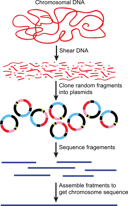
Figure 30.29. Genome sequencing using random fragments. By shearing the DNA, cloning it and sequencing all the fragments, the entire genome of a microbes can be rapidly sequencing. This method can be thought of as creating a giant jigsaw puzzle of DNA fragments. A computer is then used to help assemble the various pieces of sequenced DNA into a completed genome.
Detecting specific nucleic acids or proteins
As briefly mentioned in the section on stains in this chapter, the two strands of a complementary DNA duplex are able to hydrogen bond to each other and form a rather stable complex. A complex can also be formed between two strands that form a less-than-perfect complex, but such imperfect complexes are less stable than perfect ones. These properties form the basis of a number of highly valuable methods in molecular biology.
Let's say that you want to know if a particular DNA sequence is present in the microbe you are working on (whose genome has obviously not been sequence, or you would already know this information). You can take the DNA from your organism and digest it with a certain restriction enzyme, so that every possible cut is made in that DNA. The DNA is then run on an agarose gel. Now because of the phosphate backbone, all nucleic acid molecules have the identical charge per unit length, so the only reason that they might migrate differently is if they have a different length. Therefore in an agarose gel, the large fragments migrate much less than the small ones. After turning off the current, one can stain the DNA in the gel and see a pattern of many different bands, Go back and look at Figure 28.27 for an example).
But how can you ask if the DNA region you are interested in is present in that mess of bands? You take the gel above and transfer the DNA directly to a piece of membrane, to which it sticks in the identical pattern that it existed in the gel as shown in Figure 28.30. . Most of these methods begin with transferring the contents that have been separated by the gel onto some type of membrane that will hold either the nucleic acid or the protein. The finished gel is laid onto a membrane and then sandwiched between two pieces of filter paper. This is then hung in a buffer and a second eletric field is applied that causes the protein or nucleic acid to migrate out of the gel and get stuck on the membrane. This method is called a Southern blot (DNA), a Northern blot (RNA) or a Western blot (protein). This technique was first pioneered by the British biologist Edwin Southern, and it was named after him. Subsequent scientists who worked out conditions for RNA and protein had a bit of fun by naming them in reference to Southern.
Once your molecule of interest is blotted to a membrane, a detection reaction is then run. For detection of specific proteins, antibodies are added to the blot that bind only to the protein of interest. These antibodies have either an attached dye or some other feature that allows the detection of their position and therefore of the target protein.
For nucleic acids, you take a small fragment of DNA for the region that you care about and you tag it in some way - maybe with radioactivity or maybe with certain chemicals - and let this wash over the membrane. The tagged fragment stick tightly, or hybridize, when it finds a complementary strand that is perfect, and sticks weakly where there is a complementary strand that is only somewhat similar. Then you wash off the fragments that have not stuck. By washing under conditions of higher temperature or with formamide, termed high-stringency conditions, you can demand that only perfect or near perfect matches stay on the filter. There might be cases, however, where you want to also see some imperfect matches as well, so lower stringency conditions are used. Finally, you detect the location of the tagged fragment (and therefore the position of the complementing piece). If the tag was radioactive, the detection might use film or a special machine, but other tags have their own detection methods. The position and strength of the signal can be used to determine the fragment size, the abundance and the degree of match to the tagged fragment. Figure 28.30 is a video of the Southern Blot technique
Figure 30.30. The Southern Blot Technique. This is a method of detecting certain DNA fragments in a system.
DNA Arrays
With the advent of genome sequencing and microtechniques borrowed from the computer industry, it has become possible to use hybridization in a rather different way. Scientists have taken the genome sequence of organisms and used PCR or chemical synthesis to make a copy of regions of the chromosome encompassing every single gene, one at a time. These separate amplified fragments are then stuck to a glass or plastic surface in a precise way. This is called a gene array and represents the entire genome of the organism. Now if one took the same sort of tagged DNA fragment described immediately above and allowed it to hybridize to this surface, washed off the poorly hybridizing material and then detected where it remained, you would see which sequences were similar or identical to the tagged fragment. Now if you think about it for a bit, this is not very useful, since you must already know all the sequences involved, so you could have done the same thing by computer. However, this gives you a notion of the method; let's now describe a more interesting use of such an array.
What if we took the microbe for which we have the array and grew it under two different conditions. Let's say that the microbe is a pathogen that is known to turn on genes for virulence in humans whenever the temperature is raised to 37 °C (because the microbe thinks it is in a human body). Now you would certainly like to know which genes were involved in virulence, since you could try to figure out how to interfere with the function of the proteins made from those genes. You therefore grow the microbe at 25 °C (where no virulence genes are expressed) and at 37 °C and you isolate the RNA. For technical reasons, the RNA molecules are reversed transcribed into DNA that is chemically tagged with two different colors for the two culture conditions. The tagged DNA sample from each culture is then hybridized to a separate DNA array, washed and the resultant patterns of hybridization are compared. Intense spots mean that the gene was being heavily expressed, while the absence of a detectable spots means that it was not expressed. An intense spot seen from cultures at both temperatures means that the gene is always heavily expressed. However, one looks for those spots that are much more intense at 37 °C than at 25 °C, as many of these will identify genes whose products are involved in virulence. Figure 28.31 you will find a nice video of the use of a DNA array
Figure 30.31. DNA arrays. DNA arrays are another method of detecting the presence of DNA or RNA fragments in a system. The advantage of a DNA array is that you can detect many with one experiment.
As with any technique, especially a technically involved one such as this, there are a bunch of critical little details that are important for proper interpretation of the results. You really cannot completely remove all of the probe sticking to inappropriate places, so there is a background of signals all over the array. This low background is not a problem for genes that are expressed at high level, since they are well above that background. However, there are important genes whose expression is never very high, such as genes that encode regulatory proteins. The level of mRNA accumulation of such genes might be only a bit above the background of the array, making it difficult to make strong conclusions about them, at least in a quantitative way. Other such technical matters mean that while this method is powerful already, there is still room for improvement.
At its best, this approach gives an unprecedented insight into the physiology of the organism at the moment in time when the mRNA was extracted. It is, in a sense, a description of what the microbe is thinking about at that time.